The Building Re-tuning Simulator (BRS) aims to simplify and streamline the process of creating a building model for the purpose of understanding the impact of control changes. Other energy modeling tools prompt the user to define the zoning and equipment for an entire building. The BRS instead focuses on defining a representative subset of the building that can either be modeled independently or can be scaled up (extrapolated) to represent the entire building, if desired. In particular, the simplifications made in the BRS are as follows:
- A single representative air-handler is modeled, with detailed controls specified. This single air-handler may be used to describe a conventional single-duct air-handler, a dual-duct air-handler, a dedicated outdoor air system (DOAS) only (in the event of a building with systems like radiant heating and cooling), or a DOAS that feeds into a conventional air-handler (single-duct or dual-duct). The cooling coil in the air-handler will provide the entirety of the cooling load to the chiller unless zone-level cooling is present and specified.
- A single floor (or portion of a floor) of a building that is potentially multistory is specified. The single floor is not meant to be one specific actual floor, but a typical floor of the building. The floor is implicitly assumed to be a middle floor; thus, any inter-floor heat transfer, including heat transfer to/from the roof or foundation of the building, is neglected.
- Up to eight zones may be used to specify the typical floor. These eight zones are meant to encapsulate the diversity of loads that come about as a result of different perimeter orientations and different space-use types. Modeling individual rooms or individual heating, ventilation, and air conditioning (HVAC) zones is not possible outside of this eight-zone limit.
In some cases, these simplifications may be excessively limiting. For example, a building may be zoned with a set of air-handlers serving the core of a building and another set serving the perimeter. A building like this would require at least two instances of the BRS; one that focuses on the core Air Handling Units (AHUs) and one that focuses on the perimeter AHUs. Other buildings may have a relatively balanced mix of single-duct and dual-duct AHUs, and again, the same guidance would apply. However, for most buildings, this simplified approach eliminates a lot of the time required to specify the building, the zoning, and the HVAC connections, and instead focuses on the controls and their impact on satisfying typical zone loads within the building and on patterns of energy consumption.
The BRS operates by importing a weather file and a set of schedules from the user, then updating node conditions as needed (temperature, flow rate, enthalpy, humidity, etc.) at each timestep according to the scheduled operation of the building and its HVAC system. The timestep can be set by the user and is ideally at least a few times per hour.
Zone Details
At the zone level, a single zone temperature is calculated at every timestep based on an aggregation of a series of zone loads (cooling loads positive; heating loads negative), plus any zone-level heating or cooling that is counteracting the zone loads to maintain the zone temperature (when applicable according to thermostat, occupancy, and plant-side lockout settings). The zone loads are as follows:
- Internal loads (lighting, plug loads, and people) are based on the specification of a zone-level peak load density and an hourly schedule that modifies that density.
- Window heat gain/loss is based on a drawn zone geometry map that defines wall area (AW), a specified window-wall ratio, and a specified solar heat gain coefficient. The solar heat gain through the windows at any hour is defined as a product of those three values as well as the global horizontal solar irradiance (IG) and finally an orientation-specific solar insolation ratio (SIR), defined as the ratio of the solar insolation rate on a vertical surface facing north, south, east, or west to IG. IG comes directly from the weather file, while the SIR is interpolated from a lookup table based on the orientation and latitude. The lookup table was generated from a series of EnergyPlus simulations (https://energyplus.net/) reporting the solar loading on vertical surfaces in the cardinal orientations.
- The wall heat gain/loss uses a standard thermal conduction calculation based on the specified exterior wall U-factor. The driving temperature difference is based on the interior zone temperature (TZone) on one side, and the sol-air temperature (Tsol-air) on the other side. The sol-air temperature is a way of modifying the outdoor air temperature (TOA) to better incorporate the role of exterior wall solar heat gain in thermal conduction calculations. The sol-air temperature is estimated as
Tsol-air = TOA + 0.072 * IG * SIR - 7.02
- Infiltration is calculated based on a baseline infiltration rate (at neutral building pressure) and a linear equation that modifies the infiltration based on building pressure, which is in turn estimated based on ‘excess outdoor air’ that is positive when outdoor air intake flow rates are higher than exhaust air flow rates. This approach of explicitly calculating infiltration rates as a function of building pressure differences brought about by HVAC system control is a novel feature of the BRS relative to other tools, which do not attempt to make this connection. It is, however, a connection that is needed to estimate the energy savings impacts from controls that have an impact on building pressures. The infiltration load (Qinf) is equal to the difference in temperature between the infiltration air at ambient temperature and the zone air it is displacing, multiplied by the mass flow rate(ṁinf)
and specific heat of the infiltration air (Cpinf).
Qinf = (TZone - TOA ) * ṁ inf * Cpinf
- Inter-zone load is calculated based on the zone cross-sectional boundary with other zones, an assumed inter-zone U-factor which can be modified by the user, and a driving temperature difference between the various other zones.
QZonexZoney = AZonexZoney * (TZonex - TZoney) * Uinterzone
- Supply air-driven load is load brought into the zone from the zone-level air terminal (e.g., Variable air volume- VAV box), upstream of any zone-level reheat. This load is equal to the difference in temperature between the supply air and the zone air it is displacing, multiplied by the mass flow rate (ṁSup) and specific heat of the supply air (CpSup).
QSup =(TZone - TSup) * ṁSup * CpSup
The model treats different types of zone-level heating and cooling equipment the same. The equipment is sized to meet the 99.5th percentile annual zone loads, and then heating and cooling equipment, if they exist, can run to meet thermostatically driven zone loads. The heating equipment may be a VAV box reheat coil, a fan-coil unit, a baseboard heater, a radiant slab heater, or a space heater. All that matters from the model’s perspective is the source of the heating (e.g., electric resistance, natural gas boilers, steam) the efficiency of the heating source (defined in the heating plant specification) and the zone heating loads at any timestep. The same is true for zone cooling equipment.
The zone temperature at each timestep is calculated recursively as the temperature in the previous timestep, plus a change in zone temperature due to the loads and mechanical heating/cooling in the current timestep:
Tz,t = Tz,t-1 + ( ∑QLoads + ∑QHeat,Cool) / (Az * Mz * t)
where Tz,t is the zone temperature in timestep t, QLoads are the zone heating and cooling loads described above, QHeat,Cool are the zone-level mechanical heating and cooling provided, Az is the zone area, Mz is the zone thermal mass (in units W-h/F-ftsup>2), and t is the number of timesteps per hour.
Zone airflow rates are governed by VAV box airflow response curves. Constant-volume airflow delivery (e.g., constant-volume terminal, direct-to-zone DOAS) can be simulated by setting minimum (and heating maximum) airflow setpoints to 100%. Single-duct VAV boxes can either have single maximum or dual maximum airflow control. Single maximum control means that in heating mode, the VAV box uses the same minimum airflow setpoint as in deadband mode. Then, in cooling mode, the airflow ramps up from minimum airflow to maximum airflow. The BRS allows the user to specify the zone temperature ranges (relative to the cooling thermostat setpoint) within which the box will ramp up from its minimum to maximum airflow setpoint.
For dual maximum VAV box control, in addition to the cooling response described for the single maximum, the VAV box will ramp up to a separate heating maximum airflow setpoint as the zone temperature deviates from its heating setpoint. Again, the user can specify the zone temperature ranges relative to the heating thermostat setpoint that the box will ramp up to from its minimum to its heating maximum setpoint. The user can either specify a single global minimum VAV box airflow setpoint or can set the minimums zone-by-zone.
Figure 1 shows a sample airflow response to zone temperatures for a dual-maximum VAV box. In this case, the box has a heating thermostat setpoint of 72 °F, a cooling thermostat setpoint of 72.5 °F, a minimum airflow setpoint of 40% of its calculated design cooling maximum, and a heating maximum of 60% of its design cooling maximum airflow. The cooling airflow rate begins to ramp up at 0.2 °F below the cooling thermostat setpoint and reaches its maximum at 0.5 °F above the cooling thermostat setpoint. A similar ramp is programmed for heating.
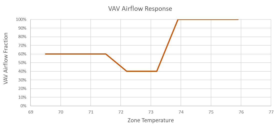 Figure 1: Dual-Maximum Airflow Control
Dual-duct VAV boxes have airflow control from each duct that act independently of one another. The user specifies a maximum cooling airflow percentage and a maximum heating airflow percentage, relative to the box’s calculated design airflow. A minimum airflow setpoint (percentage) is also specified, and this setpoint affects the duct that supplies ventilation. Ducts that do not supply ventilation go to zero airflow when their conditioning is not required. In some configurations, both ducts may provide ventilation air. In this case, the user specifies which duct provides the ventilation air when the zone is in its thermostat deadband. Finally, a control strategy is specified—either mixing or snap-action. Mixing control ramps the cold deck up at the same time that the hot deck ramps up while zone temperature increases. Snap-action control switches from the use of the hot deck to the cold deck only as the zone temperature increases. Figure 2 shows an example of
mixing airflow control, and Figure 3 shows an example of snap-action airflow control for a VAV box with ventilation in both ducts and cold-duct ventilation in the thermostat deadband. In both figures, the hot deck airflow is represented in red and the cold deck airflow is represented in blue.
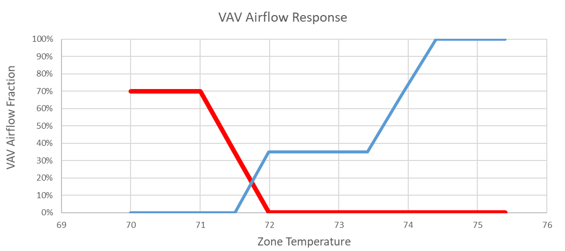 Figure 2: Mixing control with ventilation from both ducts and cold duct ventilation in thermostat deadband
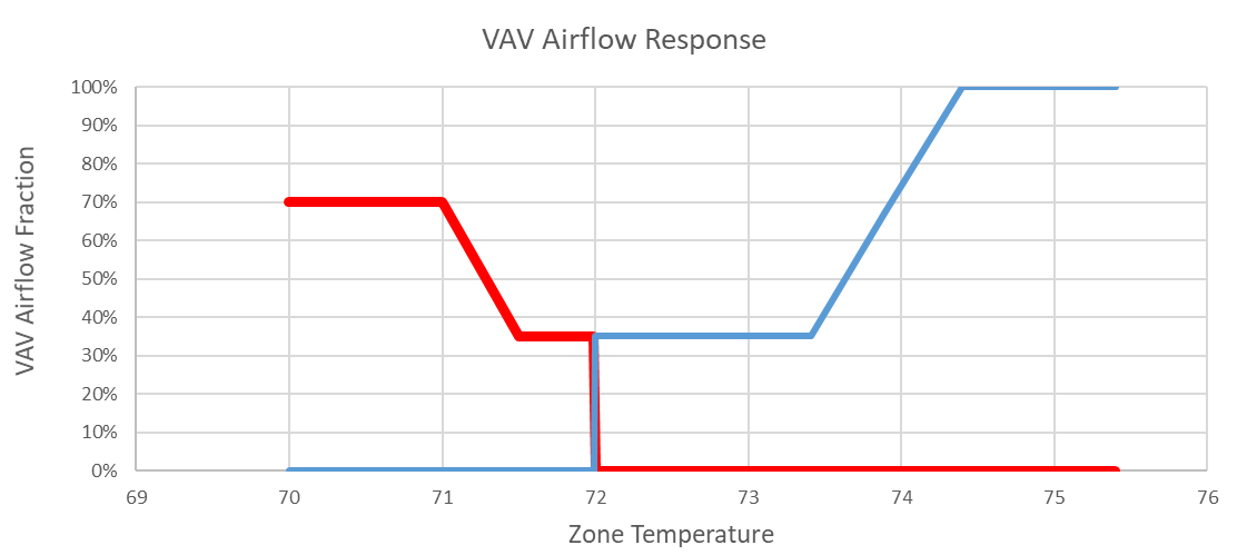 Figure 3: Snap-action control with ventilation from both ducts and cold duct ventilation in thermostat deadband
Air-Handler
The air delivered to the zones is split from a single air-handler, as previously described. The air-handler configuration (DOAS, single-duct, dual-duct, or combination) is specified by a process of inclusion or elimination of components. For example, there are five potential components in the DOAS section of the air-handler (heat recovery, heating coil, coiling coil, fan, and humidifier). If there is no DOAS, all of these components can be removed. There are also two potential heating coils, one on either side of the cooling coil so that the order (heating then cooling or cooling then heating) of the coils can be specified. Specifying components in both the DOAS and main AHU section simulates a configuration where conditioned air from one or more DOAS systems is split and sent to the outdoor air intakes of the various building AHUs. To make this work approximately as it would in a real building, the economizer control should be set to “off” and a fixed flow rate
of outdoor air should be set at the mixing box, approximating a typical flow rate from all DOAS units combined. Dual-duct configurations can be specified by including a heating coil or fan in the hot deck section of the AHU. Each component has different specified fields, as follows.
- Heating Coils:
- Setpoint type: Either a fixed setpoint at the outlet of the heating coil can be specified, or a control that maintains a downstream setpoint (DOAS SAT setpoint, AHU SAT setpoint, hot deck SAT setpoint) can be specified. In the latter case, the coil will take into consideration how each of the downstream components will add or subtract heat, and a temperature will be targeted that seeks to maintain the downstream setpoint.
- Leaking coil: A leaking coil can be modeled by specifying a fixed temperature gain across the coil when the heating system is enabled (when the AHU is running and outdoor air temperatures are below an optional outdoor-air temperature-based heating coil lockout setpoint).
- Cooling Coils:
- Setpoint type: Either a fixed setpoint at the outlet of the cooling coil can be specified, or a control that maintains a downstream setpoint (DOAS SAT setpoint, AHU SAT setpoint) can be specified. In the latter case, the coil will take into consideration how each of the downstream components will add or subtract heat, and a temperature will be targeted that seeks to maintain the downstream setpoint.
- Leaking coil: A leaking coil can be modeled by specifying a fixed temperature loss across the coil when the cooling system is enabled (when the air-handler is running and outdoor air temperatures are above an optional outdoor-air temperature-based cooling coil lockout setpoint).
- Humidifier:
- Location: The humidifier can be located in six different locations within the DOAS, AHU section, and return air section.
- Relative humidity setpoint: The relative humidity setpoint is set at the return air node downstream of the return fan, if any.
- Outdoor air temperature lockouts: High and low outdoor air temperature lockouts of the humidifier can be specified.
- Fuel source: The fuel source can either be steam or electric.
- Fan:
- Temperature rise: Typical temperature rise across the fan, which can often be determined through Building Automation System graphics/trends on temperature sensors in the AHU section.
- Efficiency: The user has three qualitative choices that can be made based on observations about the age and state of the fan. Medium (50% efficiency) is the default, with low (40%) and high (60%) as alternative options.
- Observed duct static pressure: Used to make adjustments to fan pressure rise as the duct static pressure setpoint changes and in turn changes the total fan pressure rise. The fan temperature rise should correlate linearly with total pressure rise.
- Total static pressure: Total pressure rise across the fan.
- Outdoor air mixing box:
- Minimum outdoor air (OA) control type: User can select from “minimum OA fraction,” “minimum OA CFM,” “minimum OA fraction of design flow,” and DCV. “Minimum outdoor air fraction” produces a variable CFM in minimum outdoor air mode to maintain a constant outdoor air fraction. This is typical of units that do not have outdoor airflow sensors or controls and instead use fixed minimum outdoor air damper commands. “Minimum OA fraction of design flow” controls to a constant minimum outdoor air CFM, but the sizing of this minimum flow is made in this case as a fractional multiplier of the design AHU airflow rate. Finally, “DCV” is demand control ventilation and allows a linear reset of the minimum outdoor air fraction based on return air CO2 concentrations, which are calculated based on people densities, space volume outdoor/exhaust airflows, and infiltration flow rates.
- Economizer present/control: The user can specify whether or not the economizer is present, and if so, what economizer control is used. Options include “fixed dry bulb,” “fixed enthalpy,” “differential dry bulb,” and “differential enthalpy.” Outdoor air temperature lockouts of the economizer can be specified (whether or not the choice is “fixed dry bulb”).
The air conditions (temperature, humidity, enthalpy, and flow rate) are calculated sequentially through each node (inlet and outlet of each component) starting upstream at the outdoor air intake and moving downstream to the supply air delivery to the zones. In some cases, the node temperatures require looking ahead to downstream components’ setpoints and the operation of other downstream components. For example, if there is a heating coil with a cooling coil and a fan downstream before the supply air discharge, if the cooling coil has a 3 °F leak, and if the fan has a 2 °F temperature rise, then the heating coil should target an outlet air temperature that is 1 °F warmer than the supply air temperature.
The BRS uses a set of psychrometric functions to calculate the enthalpy, and in some cases the temperature and humidity downstream of each component. For heating coils, cooling coils, and humidifiers, the energy consumed at the component can be simply calculated as the product of the mass flow rate and the difference in enthalpy between the inlet node and outlet node.
The AHU will shut off outside a specified HVAC operating schedule unless the temperature in one or more of the zones drifts outside of the unoccupied thermostat heating or cooling setpoints, in which case the AHU will operate until the thermostats are satisfied again. There is an option for the user to specify that specific zones have the ability to perform after-hours heating without the use of the air-handler (for example, through the use of baseboard heaters or fan-coil units). When these zones fall below their heating night setback setpoints, the AHU will remain off.
Several setpoints at the AHU level can accept ‘resets’ or feedback control of their setpoint values. These include the main AHU/cold deck static pressure setpoint, the hot deck static pressure setpoint, the DOAS supply air temperature and the AHU supply air temperature setpoints, and the hot deck supply air temperature setpoint. There are two types of resets available: linear resets and trim-and-respond resets. Linear resets involve explicitly setting the setpoint based on the current value of the feedback variable. There is a minimum value and a maximum value of the setpoint associated with corresponding minimum and maximum values of the feedback variable (or vice versa). In between, the setpoint is interpolated based on the progress between the minimum and the maximum levels of the feedback variable. Trim-and-respond resets likewise have a minimum and maximum value of the setpoint, but use a recursive strategy that incrementally adjusts the setpoint until the feedback
variable approaches a target value. Available feedback variables for these resets include:
- outdoor air temperature
- zone cooling demand (an average value among all the zones, calculated for individual zones as 0 when the zone temperature is less than 0.7 °F below the zone cooling thermostat setpoint and ranging up to 100 when the zone temperature is more than 0.3 °F above the zone cooling thermostat setpoint)
- zone heating demand
- zone cooling minus zone heating demand
- maximum cooling demand
- return air temperature
- supply fan speed
- average zone damper
- maximum zone damper
Cooling Plant
The cooling plant imports cooling loads primarily from the air-handler, but also from zone-level hydronic cooling equipment if it exists. In the case that direct expansion (DX) coils are specified as the cooling source for the building, no cooling plant will be simulated. If district cooling is specified as the cooling source, the cooling plant will be used to aggregate the cooling loads and simulate the building chilled water pumps. Otherwise, the following are optional components in the cooling plant, along with the inputs required for each. In many cases, the inputs themselves are optional, as specified below. If inputs are not specified, they will be chosen as indicated either with a default or autosized value.
- Chillers (up to 4)
- Capacity for each chiller (required)
- Speed – variable or constant (required)
- Efficiency – COP or kW/ton rated (optional) default: 0.7 kW/ton
- Minimum part load ratio (optional) default: 20%
- Part load ratio for stage-up and stage-down (required)
- Primary pumps (up to four). Note that these are constant-speed pumps that are dedicated one per chiller. Single-loop pumping configurations should be specified as secondary pumps.
- Nameplate power (optional) autosized at: (Water Flow gpm-118.7)/20.9
- Water flow (optional) autosized at: 2.2 x Chiller Tons
- Efficiency – (optional) default: 60%
- Rated head (optional) default: 30 ft w.c.
- Secondary pumps (up to four). These pumps serve the building loop.
- Nameplate power (required)
- Water flow (optional) autosized at: total pumping system sizing: 2.2 x maximum building demand tons (if no chillers) or 2.2 x Total chiller tons
- Efficiency – (optional) default: 60%
- Rated head (optional) default: 60 ft w.c.
- Minimum part load ratio (PLR) (optional) default: 25%
- PLR for stage-up and stage-down (required)
- Condenser pumps (up to four). Note that these are constant-speed pumps that can either be specified as dedicated one per chiller, or staged up based on demand (more condenser water flow is needed than is being supplied by the current number of condenser pumps).
- Nameplate power (optional); autosized at: (water flow gpm − 118.7)/20.9
- Water flow (optional); autosized at: total pumping system sizing: 2.2 × maximum building demand tons (if no chillers) or 2.2 × total chiller tons
- Efficiency – (optional); default: 60%
- Rated head (optional); autosized at: nameplate power [hp] × pump efficiency × 1,714/ water flow [gpm].
- Cooling towers (up to four). Note that these are constant-speed pumps that can either be specified as dedicated one per chiller, or staged up based on demand (more condenser water flow is needed than is being supplied by the current number of condenser pumps).
- Fan power (optional); autosized (kW) at: 0.0369 × chiller tons
- Capacity (tons) (optional); autosized at: 1.33* chiller tons
- Tower type (required): Single speed, two speed, and variable speed
- PLR for stage-up and stage-down (required).
Chillers are modeled using the same approach as in EnergyPlus. The rated Coefficient of Performance (COP) is used to define an energy input ratio (EIR), which is the dimensionless ratio of the input power to the compressor divided by the input power at rated conditions (rated capacity, rated evaporator outlet temperature TChW,o,rated, rated condenser inlet temperature TCW,i,rated). The EIR is modified by two curves. The first curve (EIR function of temperature, or EIRFT) modifies the EIR as a function of the current evaporator outlet temperature, TChW,o, and the current condenser inlet temperature, TCW,i. TCW,i is the outdoor air temperature for air-cooled chillers and the condenser water inlet temperature (cooling tower outlet temperature) for water-cooled chillers. The EIRFT curve is a six-coefficient regression equation:
EIRFT=a1+a2 * TChW,o+a3 * TChW,o2+a4 * TCW,i+a5 * TCW,i 2+a6 * TChW,o * TCW,i
The second curve is the EIR function of the PLR curve, or EIRFPLR. This curve modifies the EIR based on its part load operation. The EIR is defined as the ratio of the current chiller load (tons), divided by the rated capacity of the chiller. The EIRFPLR curve is a simple quadratic curve:
EIRFT=b1+b2 * PLR+b3 *PLR2
The chiller power consumption at any condition can then be calculated as:
P_Ch=Capacityrated/COPrated * EIRFT * EIRFPLR
A third curve (capacity function of temperature, or CAPFT) is used to modify the chiller’s rated capacity based on changing evaporator and condenser temperatures. The curve takes the same form as the EIRFT curve:
CAPFT=c1+c2 * TChW,o+c3 * TChW,o2+c4 * TCW,i+c5 TCW,i2+c6 * TChW,o * TCW,i
Default coefficients for each of the three curves are used for both constant-speed and variable-speed chillers for the three curves. Constant-speed and variable-speed coefficients are shown in Table 1 and Table 2, respectively.
Table 1: Constant-speed chiller coefficients.
|
1 |
2 |
3 |
4 |
5 |
6 |
| EIRFT (a) |
0.732 |
‒0.0246 |
0.000294 |
0.00689 |
0.000116 |
‒0.000218 |
| EIRFPLR (b) |
0.118 |
0.502 |
0.309 |
| CAPFT (c) |
‒2.374 |
0.0946 |
‒0.00194 |
0.0328 |
‒0.000649 |
0.00127 |
Table 2: Variable-speed chiller coefficients.
|
1 |
2 |
3 |
4 |
5 |
6 |
| EIRFT (a) |
0.732 |
-0.0246 |
0.000294 |
0.00689 |
0.000116 |
‒0.000218 |
| EIRFPLR (b) |
0.0977 |
0.249 |
0.654 |
| CAPFT (c) |
‒0.625 |
‒0.0379 |
‒0.000547 |
0.0754 |
‒0.00105 |
0.00140 |
Setpoints for TChW,o and TCW,i can each be reset in the tool as re-tuning measures. TChW,o can either be set as constant or can be reset linearly based on chilled water valve position. TCW,i can either be set as constant or can be reset as a constant offset from the outdoor air wet bulb temperature, with minimum and maximum limits.
Variable-speed pump power is calculated based on the following equation:
Ppump=Ppump,rated * DPpump /DPpump,rated (0.573 * PLRpump-0.301 * PLRpump2+0.735 * PLRpump3 )
Ppump,rated is set as half of the nameplate pump power, as a heuristic. The pump differential pressure, DPpump, can either be set as a constant or reset as a re-tuning measure as a function of the chilled water coil valve position.
PLRpump is the ratio of the pump water flow rate to the rated pump water flow rate.
Cooling tower power consumption is calculated according to the following equation:
Ptower=PTower,rated * (0.00153+0.0052 * PLRtower+1.1086 * PLRtower2-0.116 * PLRtower3 )
PLRtower is the ratio of the cooling tower airflow to the rated airflow. The cooling tower airflow is calculated as:
Vtower=Qcond /( 4.5 * (Htower,air,out-Htower,air,in ) )
In the case of two-speed tower fans, Ptower is set to half of PTower,rated when PLRtower is greater than 0 and less than 0.5. If PLRtower is greater than 0.5, Ptower is set to PTower,rated.
Heating Plant
The heating plant imports heating loads from the air-handler and from zone-level heating equipment. In the case that DX coils are specified as the heating source for both the AHU and the zone-level equipment, no heating plant will be simulated. If district steam is specified as the heating source, the heating plant will be used to aggregate the heating loads and simulate the building hot water pumps. Otherwise, the following are optional components in the heating plant, along with the inputs required for each:
- Boilers (up to eight)
- Boiler type (required): non-condensing or condensing
- Sizing [mmBtu/hr] (required)
- Design boiler efficiency (optional): default: 80% for non-condensing and 91% for condensing boilers
- PLR for stage-up and stage-down (required)
- Primary pumps (up to eight). Note that these are constant-speed pumps that are dedicated one per boiler. Single-loop pumping configurations should be specified as secondary pumps.
- Nameplate power (optional); autosized at: water flow [gpm] 0.00473/pump efficiency
- Rated water flow (optional); autosized at: boiler size [mmBtu/hr] × 2,000/design coil dT
- Efficiency – (optional); default: 60%
- Rated head (optional); default: efficiency × nameplate power × 1,714/rated water flow.
- Secondary pumps (up to three). These pumps serve the building loop.
- Nameplate power (optional); autosized at: 0.0207*Rated flow/pump efficiency
- Water flow (optional); autosized at: maximum building heating load × 2,000/design coil dT
- Efficiency – (optional); default: 60%
- Rated head (optional); default: efficiency × nameplate power × 1,714/rated water flow
- Minimum PLR (optional); default: 25%
Several additional inputs are needed for the hot water loop:
- Design coil delta T: default: 15 °F
- Secondary loop line loss coefficient (c_loss): default: 0.5
This input is used to calculate loss of heat to unconditioned spaces. This value can be later changed in the calibration process. Whenever the pumps are running, the boiler or district hot water loop will have to compensate for the following amount of heat:
Qloss,HW = ((THW-75) QHW,maxload * closs) / 1000
Where T_HW is the hot water temperature setpoint, and Q_(HW,maxload) is the maximum building hot water load.
- Design loop differential pressure (optional): Can be set by the user or autosized either as the constant differential pressure specified in the baseline or the maximum differential pressure specified in a baseline differential pressure reset. Note that the differential pressure reset uses the average hot water coil valve as the feedback variable in a linear reset.
- Simultaneous heating and cooling (%): This value specifies a plant-side mix heating and cooling as a percent of the smaller of the two loads. For example, if there is 100 kW of heating load and 200 kW of cooling load in a building at a certain timestep and this value is set to 10%, an additional load of 10 kW will be sent to the boiler and the chiller loads that are conceptually cancelled out somewhere in the building.
QSimHC=csimHC * min( HWLoad , ChWLoad )
T_HW can be set as a constant value or can accept a linear reset with either the outdoor air temperature or the average hot water coil valve as the feedback variable for the reset.
For non-condensing hot water boilers, the fuel heat input is calculated as follows:
Q
B,heat = ( ( Q
HW + Q
loss,HW + Q
SimHC ) ) / ɳ
B,rated
Where ɳB,rated is the rated boiler efficiency.
For condensing boilers, the efficiency is a more dynamic function of the PLR, PLRB, and the boiler hot water return temperature, TB,R. A nine-coefficient regression equation is used to calculate the instantaneous efficiency and boiler fuel heat input:
QB,heat = ( ( QHW + Qloss,HW + QSimHC ) ) / ( PLRB2 (a1 * TB,R2 + a2 * TB,R + a3 ) + PLRB * ( b1 * TB,R2 + b2 * TB,R + b3 )+( c1 * TB,R2 + c2 * TB,R + c3 ) )
The coefficients for the regression equation are listed in Table 3.
Table 3: Regression coefficients for condensing boiler efficiency calculations.
|
a |
b |
c |
| 1 |
0.00000589 |
‒0.00000736 |
0.00000884 |
| 2 |
‒0.00216 |
0.00309 |
‒0.00323 |
| 3 |
0.189 |
‒0.312 |
1.003 |
Hot water constant-speed and variable-speed pump power is calculated the same way as for chilled water pumps.